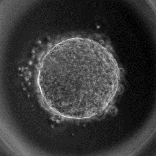
Forces and pressure play a key role in the development of an organism. These forces that are generated by the cells can act upon other cells in concert to yield dramatic changes in the architecture of a tissue. Forces may cause a tissue to stretch or rotate. Likewise, the internal pressure within the cells may cause the tissue to bulge or contract. Without precise regulation of forces and pressure by the cells it is not hard to imagine that the developmental processes will be severely impacted. Therefore, biologists and biophysicists who are studying animal development often need a measure of the distribution of forces and pressure in a tissue over time.
There are experimental methods for measuring forces. In “laser ablation” a high-powered laser beam can be used to ablate junction(s) between two or more cells that are under tension. The recoil velocity can be used to determine the magnitude of tension. Imagine cutting a guitar string that is under high tension. Once snapped it will spring back. The process is highly invasive, that is the junction in query has to be severed, rendering it less useful to study forces in a spatio-temporal manner.
In this post I would like to share with you the notion of inferring forces and pressure in a tissue using images. This technique, now commonly known as “Force Inference” was proposed by Ishihara and Sugimura (Journal of Theoretical Biology, 2012) as well as Brodland (2014). Force Inference allows us to determine forces without having to destroy tissues. And the idea is pretty simple. A cell is delimited by the junctions (edges) enclosing it and an edge can be represented by a line drawn between two vertices. We assume that a tissue at any given moment is in quasi-equilibrium and consequently the forces acting on the vertices sum to zero. Such an assumption makes sense since morphological changes in tissues occur over a long time-scale. The inertial and viscous effects are negligible. The forces acting on a vertex are both due to tension acting along the cell-cell junctions and the internal pressure of the cell.
Here is a Mathematica implementation that uses force balance over all vertices of an epithelia (sheet of cells) to determine the unknown tension and pressure. Note that the forces and pressure determined from this method only yields a relative estimate of the unknowns and not an absolute one. The script is based on the approach proposed by Ishihara
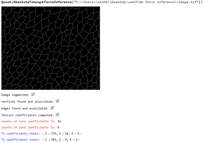
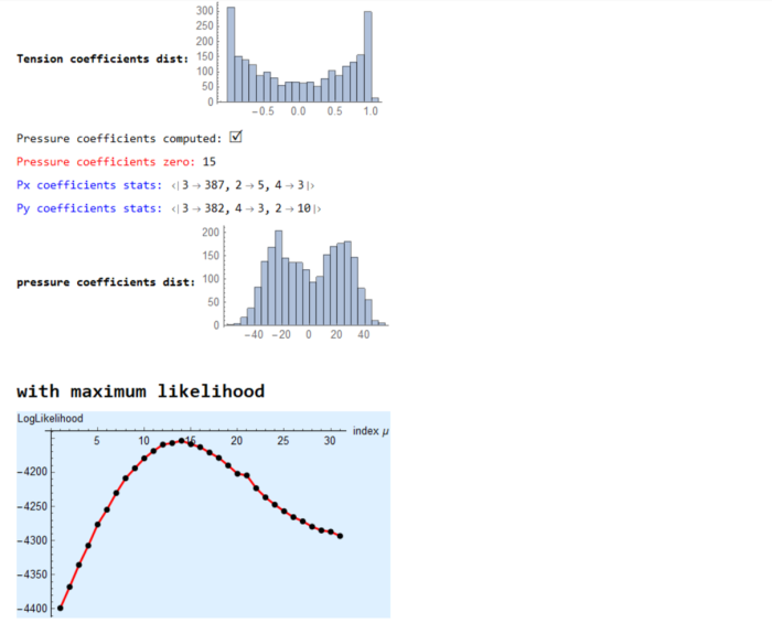
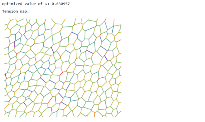

(* ::Package:: *)

(* ::Section:: *)
(*Associated Functions*)


segmentImage[binarizedMask_?ImageQ,opt:"ConnectedComponents"|"Watershed":"Watershed",
threshCellsize_:\[Infinity]]:= Module[{seg,areas,indexMaxarea,maxArea,indsmallareas={},$ind},
seg = Switch[opt,"ConnectedComponents",
(* assuming we input 0 as foreground and 1 as background. ConnectedComponents is a more general segmentation framework *)
MorphologicalComponents[ColorNegate@binarizedMask, CornerNeighbors->False],
"Watershed",(* for epithelial cells *)
WatershedComponents[binarizedMask, CornerNeighbors->False]
];
areas=ComponentMeasurements[seg,"Area"];
{indexMaxarea,maxArea}=First@MaximalBy[areas,Last]/.Rule-> List;
indsmallareas = Keys@Cases[areas,HoldPattern[_-> 1.]];
If[maxArea >= threshCellsize||indsmallareas!= {},
$ind={indexMaxarea}~Join~indsmallareas;
seg=ArrayComponents[seg,Length@areas,Thread[$ind->0]]
];
seg
];


Options[associateVertices]= {"stringentCheck"-> True};
associateVertices[img_,segt_,maskDil_:2,OptionsPattern[]]:= With[{dim =Reverse@ImageDimensions@img,
stringentQ=OptionValue["stringentCheck"]},
Module[{pts,members,vertices,nearest,vertexset,likelymergers,imagegraph,imggraphweight,imggraphpts,vertexpairs,
posVertexMergers,meanVertices,Fn},
pts = ImageValuePositions[MorphologicalTransform[img,{"Fill","SkeletonBranchPoints"}], 1]; (* finding branch points *)
members = ParallelMap[Block[{elems},
 elems = Dilation[ReplaceImageValue[ConstantImage[0,Reverse@dim],#->1],1];
 DeleteCases[Union@Flatten@ImageData[elems*Image[segt]],0.]
 ]&,pts];
vertices = Cases[Thread[Round@members-> pts],HoldPattern[pattern:{__}/;Length@pattern >= 2 -> _]];
(* finding vertices with 2 or more neighbouring cells *)
nearest = Nearest[Reverse[vertices, 2]]; (* nearest func for candidate vertices *)
Fn = GroupBy[MapAt[Sort,(#-> nearest[#,{All,3}]&/@Values[vertices]),{All,2}],Last->First,#]&;
Which[Not@stringentQ,
 (* merge if candidate vertices are 2 manhattan blocks away. Not a stringent check for merging *)
 KeyMap[Union@*Flatten]@Fn[List@*N@*Mean]//Normal,
 stringentQ,
 (* a better check is to see the pixels separating the vertices are less than 3 blocks *)
 vertexset = Fn[Identity];
 (* candidates for merging*)
 likelymergers = Cases[Normal[vertexset],PatternSequence[{{__Integer}..}-> i:{__List}/;Length[i]>= 2]];
 (*defining graph properties of the image *)
 imagegraph = MorphologicalGraph@MorphologicalTransform[img,{"Fill"}];
 imggraphweight = AssociationThread[(EdgeList[imagegraph]/.UndirectedEdge->List )-> PropertyValue[imagegraph,EdgeWeight]];
 imggraphpts = Nearest@Reverse[Thread[VertexList[imagegraph]-> PropertyValue[imagegraph,VertexCoordinates]],2];
 (* corresponding nodes on the graph *)
 vertexpairs = Union@*Flatten@*imggraphpts/@(Values[likelymergers]);
 (* find pairs < than 3 edgeweights away, take a mean of vertices and update the association with mean position *)
 posVertexMergers = Position[Thread[Lookup[imggraphweight,vertexpairs]< 3],True];
 If[posVertexMergers != {},
  meanVertices=MapAt[List@*N@*Mean,likelymergers,Thread[{Flatten@posVertexMergers,2}]];
  Scan[(vertexset[#[[1]]]=#[[2]])&,meanVertices]
  ];
  KeyMap[Union@*Flatten]@vertexset//Normal]
  ]
];


(* ::Section:: *)
(*Force Inference*)


plotMaps[p_,segmentation_,edgeImg_,maxcellLabels_,dimTx_,vertexToCells_,
vertexCoordinatelookup_,edgeLabels_]:=Module[{cellToVertexLabels,cellToAllVertices,ptsEdges,k,v,ord,edgeptAssoc,poly,pts,
mean,ordering,orderpts,tvals,cols,pvals,removecollabels,collabels,pressurecolours},

cellToVertexLabels= Reverse[vertexToCells,2];
cellToAllVertices= GroupBy[Flatten[Thread/@cellToVertexLabels],First-> Last];
(* polygons *)
ptsEdges ={{1,1},Reverse@Dimensions[segmentation],{Last[Dimensions@segmentation],1},{1,First[Dimensions@segmentation]}};
{k,v}={Keys@#,Values[#][[All,2]]}&@ComponentMeasurements[segmentation,{"AdjacentBorderCount","Centroid"},#==2&];
ord=Flatten[Function[x,Position[#,Min[#]]&@Map[EuclideanDistance[#,x]&,ptsEdges]]/@v];
edgeptAssoc=Association[Rule@@@Thread[{k,ptsEdges[[ord]]}]];
poly=(
pts=vertexCoordinatelookup/@cellToAllVertices[#];
If[MemberQ[k,#],AppendTo[pts,edgeptAssoc[#]],pts];
mean=Mean[pts];
ordering=Ordering[ArcTan[Last@#-Last@mean,First@#-First@mean]&/@pts];
orderpts=pts[[ordering]];
Polygon@Append[orderpts,First@orderpts]
)&/@Range[maxcellLabels];

tvals=Rescale@p[[1;;Last@dimTx]];
cols=ColorData["Rainbow"][#]&/@tvals;
Print["Tension map:"];
Print[Graphics[{Thickness[0.005],Riffle[cols,Line/@Values@edgeLabels]}]];
pvals=p[[ Last[dimTx]+1;;]];
removecollabels=Keys@ComponentMeasurements[segmentation,"AdjacentBorders",Length[#]>0&];
collabels=Complement[Range@maxcellLabels,removecollabels];
pressurecolours=ColorData["Rainbow"][#]&/@Rescale[(pvals[[collabels]])];
Print["Pressure map:"];
Print@Show[Graphics@Riffle[pressurecolours,poly[[collabels]]],edgeImg];
]


(* maximize Log-likelihood function *)
maximizeLogLikelihood[spArrayX_,spArrayY_,dimTx_,dimPx_]:= Module[{range=10.0^Range[-1.5,1.5,0.1],sol,spA,spg,spB,n,m,spb,\[Tau],
SMatrix,Q,R,H,h,logL,\[Mu],p},
Print[Style["\nwith maximum likelihood",Bold,18]];
sol=With[{ls=range},
(*spA=SparseArray@(Join[spArrayX,spArrayY]);*)
spA=SparseArray@(Flatten[Transpose[{spArrayX,spArrayY}],1]);
spg=SparseArray@(ConstantArray[1.,Last@dimTx]~Join~ConstantArray[0.,Last@dimPx]);
spB=SparseArray@DiagonalMatrix[spg];
n=First@Dimensions@spA;
m=(Length[#]-Total@#)&@Diagonal[spB\[Transpose].spB];
With[{DimspB=First[Dimensions@spB]},
spb=SparseArray@ConstantArray[0.,First[Dimensions@spA]];
Table[(\[Tau]=Sqrt[\[Mu]];
SMatrix=SparseArray@(Map[Flatten]@Transpose[{Join[spA,\[Tau] spB],Join[spb,\[Tau] spg]},{2,1}]);
{Q,R}=SparseArray/@QRDecomposition[SMatrix];
R=DiagonalMatrix[Sign[Diagonal@R]].R;
H=R[[;;#,;;#]]&@DimspB;
\!\(\*OverscriptBox[\(h\), \(\[RightVector]\)]\)=R[[;;#,#+1]]&@DimspB;
h=R[[#+1,#+1]]&@DimspB;
logL=-(n-m+1)*Log[h^2]+Total[Log[Diagonal[\[Mu] (spB\[Transpose].spB)]["NonzeroValues"]]]-
2*Total[Log[Diagonal[H[[1;;-2,1;;-2]]]["NonzeroValues"]]]
),{\[Mu],ls}]
]
];
Print[ListPlot[{sol,sol},Joined-> {True,False},PlotStyle->{{Red,Thick},{PointSize[0.02],Black}},AxesStyle->{{Black},{Black}},
AxesLabel->{"index \[Mu]","LogLikelihood"},Background->LightBlue]];
\[Mu]=Keys@@MaximalBy[Thread[range-> sol],Values,1];
Print["optimized value of \[Mu]: ",\[Mu]];
\[Tau]=Sqrt[\[Mu]];
With[{DimspB=First[Dimensions@spB]},
SMatrix=SparseArray@(Map[Flatten]@Transpose[{Join[spA,\[Tau] spB],Join[spb,\[Tau] spg]},{2,1}]);
{Q,R}=SparseArray/@QRDecomposition[SMatrix];
R=DiagonalMatrix[Sign[Diagonal@R]].R;
H=R[[;;#,;;#]]&@DimspB;
\!\(\*OverscriptBox[\(h\), \(\[RightVector]\)]\)=R[[;;#,#+1]]&@DimspB;
];
p=PseudoInverse[H].\!\(\*OverscriptBox[\(h\), \(\[RightVector]\)]\); p
];


formAndComputeMatrices[vertexCoordinatelookup_,inds_,colsOrder_,edgenum_,delV_,
vertexToCells_,vertexvertexConn_,maxcellLabels_,filteredvertices_,vertexAssoc_]:=Module[{tx,ty,tensinds,filteredvertexnum,relabelvert,
spArrayTx,spArrayTy,spArrayPx,spArrayPy,spArrayX,spArrayY,$filteredvertices},
{tx,ty}=Transpose[
With[{target=vertexCoordinatelookup[#[[2]]],source=vertexCoordinatelookup[#[[1]]]},
(target-source)/Norm[target-source]
]&/@inds];
Print["Tension coefficients computed: ",Style["\[CheckmarkedBox]",20]];
MapThread[Print[Style["counts of zero coefficients "<>#1,Red], Count[#2,0.]]&,{{"Tx: ","Ty: "},{tx,ty}}];
$filteredvertices=Complement[filteredvertices,delV];
filteredvertexnum=Length@$filteredvertices;
relabelvert=AssociationThread[$filteredvertices-> Range[Length@$filteredvertices]];
tensinds=Thread[{Lookup[relabelvert,Part[inds,All,1]],colsOrder}];
spArrayTx=spArrayTy=SparseArray@ConstantArray[0,{filteredvertexnum,edgenum}];
MapThread[(spArrayTx[[Sequence@@#1]]=#2)&,{tensinds,tx}];
MapThread[(spArrayTy[[Sequence@@#1]]=#2)&,{tensinds,ty}];
spArrayPx=spArrayPy=SparseArray@ConstantArray[0,{filteredvertexnum,maxcellLabels}];
MapThread[Print[Style[#1<> "coefficients stats: ",Blue],Counts@Map[Total@*Unitize,Normal[#2]]]&,
{{"Tx ", "Ty "},{spArrayTx,spArrayTy}}];
Print[Style["Tension coefficients dist: ",Bold],Histogram[{{},Join[spArrayTx["NonzeroValues"],spArrayTy["NonzeroValues"]]},20,
ImageSize->Small]];
Block[{neighbouringCells,bisectionlabels,bisectpts,centroid,orderingT,
vertexcoords,orderptsT,orderIndT,orderCells,kk=0,px,py},
With[{cellToVertexLabelsT= Reverse[vertexToCells,2],
edgeVertexPart=GroupBy[vertexvertexConn~Flatten~1 ,First-> Last]},
With[{cellToAllVerticesT= GroupBy[Flatten[Thread/@cellToVertexLabelsT],First-> Last]},
Do[
neighbouringCells= vertexToCells[[i,2]]; (* for vertex, the neighbouring cell labels *)
bisectionlabels=Intersection[cellToAllVerticesT[#],edgeVertexPart[i]]&/@neighbouringCells ;
If[Length[neighbouringCells]>2 && MatchQ[bisectionlabels,{Repeated[{_,_},{3,\[Infinity]}]}],
(vertexcoords=DeleteDuplicates[vertexCoordinatelookup[#]&/@Flatten@bisectionlabels];
centroid=Mean@vertexcoords;
orderingT=Ordering[ArcTan[Last@#-Last@centroid,First@#-First@centroid]&/@vertexcoords];
orderptsT=vertexcoords[[orderingT]];
orderIndT=Partition[Lookup[vertexAssoc,Append[orderptsT,First@orderptsT]],2,1];
 orderCells =
Last@@@Position[(x\[Function] Map[Intersection[x,#]&,orderIndT])/@(cellToAllVerticesT[#]&/@neighbouringCells),x_/;Length[x]==2];
neighbouringCells=neighbouringCells[[orderCells]];
bisectpts=Map[vertexCoordinatelookup,orderIndT,{2}];
{px,py}=Transpose[{(#[[2,2]]-#[[1,2]])/2,-(#[[2,1]]-#[[1,1]])/2}&/@bisectpts];
If[MemberQ[px,0.]||MemberQ[py,0.],kk++];
{px,py})
];
Scan[(spArrayPx[[ Sequence@@#[[1]] ]]=#[[2]])&,Thread[Thread[{relabelvert@i,neighbouringCells}]-> px]];
Scan[(spArrayPy[[ Sequence@@#[[1]] ]]=#[[2]])&,Thread[Thread[{relabelvert@i,neighbouringCells}]-> py]],
{i,$filteredvertices}]
]
];
Print["Pressure coefficients computed: ",Style["\[CheckmarkedBox]",20]];
Print[Style["Pressure coefficients zero: ",Red],kk ];
];
MapThread[Print[Style[#1<> "coefficients stats: ",Blue],Counts@Map[Total@*Unitize,Normal[#2]]]&,
{{"Px ", "Py "},{spArrayPx,spArrayPy}}];
Print[Style["pressure coefficients dist: ",Bold],
Histogram[{{},Join[spArrayPx["NonzeroValues"],spArrayPy["NonzeroValues"]]},ImageSize->Small]];
spArrayX=Join[spArrayTx,spArrayPx,2];
spArrayY=Join[spArrayTy,spArrayPy,2];
{spArrayX,spArrayY,Dimensions[spArrayTx],Dimensions[spArrayPx]}
]


ForceInference[filename_]:=Module[{Img,segmentation,maxcellLabels,cellsToVertices,vertexnum,edges,smalledges,maxedgeLabels,
edgeEndPoints,nearest,nearestedgeEndPoints,edge2pixLabels,pos,oldCoords,vertexAssoc,vertexToCells,filteredvertices,filteredvertexnum,
relabelvert,edgeLabels,edgenum,spArrayTx,spArrayTy,vertexCoordinatelookup,vertexpairs,vertexvertexConn,inds,edgelabelToVert,delV,
vertToedges,edgeImg,colsOrder,p,spArrayX,spArrayY,dimTx,dimPx},

LaunchKernels[];
Img= ColorConvert[Import[filename],"Grayscale"];
Print[Image[Img,ImageSize->Medium]];
segmentation = segmentImage[Img];
Print["Image segmented: ", Style["\[CheckmarkedBox]",20]];
maxcellLabels = Max@Values@ComponentMeasurements[segmentation,"LabelCount"];
cellsToVertices = associateVertices[Binarize@Img,segmentation];
Print["vertices found and associated: ", Style["\[CheckmarkedBox]",20]];
vertexnum=Length@cellsToVertices;
edges=MorphologicalComponents@ImageFilter[If[#[[3,3]] == 1 && Total[#[[2;;-2,2;;-2]],2] == 3, 1, 0]&,Img,2];
(* associate vertices with all edges. for pixel value 1 edge find two nearest pts. for all edges <3, merge the pts together;
 make changes to the cellToVertex *)
(* edges to be deleted *)
smalledges=Flatten[Position[Values@ComponentMeasurements[edges,"Count"],1|2]];
maxedgeLabels=Max@edges;
edgeEndPoints=With[{comp=Values@ComponentMeasurements[edges,"Mask"]},
ParallelTable[
If[Total[#] == 1,ImageValuePositions[#,1],
ImageValuePositions[MorphologicalTransform[#,"SkeletonEndPoints"],1]]&@Binarize@Image[comp[[i]]]
,{i,maxedgeLabels}]
];
(* for small edge: if one pixel delete *)
edges=Fold[If[Length@edgeEndPoints[[#2]]==1,#1/.#2 -> 0,#1]&,edges,smalledges];
nearest=Nearest@Flatten[Values[cellsToVertices],1];
nearestedgeEndPoints=Map[Flatten@*nearest,edgeEndPoints,{2}];
(* if edge is two pixels then put average value in the cellsToVertices: *)
edge2pixLabels=Keys@Cases[ComponentMeasurements[edges,"Count"],HoldPattern[_-> 2]];

If[edge2pixLabels!={},
(oldCoords=nearestedgeEndPoints[[#]];
pos=Position[cellsToVertices,#,Infinity]&/@oldCoords;
cellsToVertices=Fold[ReplacePart[#1,#2-> Mean@oldCoords]&,cellsToVertices,pos]
)&/@edge2pixLabels
];
edges=ArrayComponents[edges/.Thread[edge2pixLabels-> 0]];
Print["edges found and associated: ", Style["\[CheckmarkedBox]",20]];
cellsToVertices=Normal@AssociationMap[Reverse,GroupBy[cellsToVertices,Last-> First,Union@*Flatten]];
vertexnum=Length@cellsToVertices;
nearest=Nearest@Flatten[Values@cellsToVertices,1];
edgeEndPoints=Delete[edgeEndPoints,Partition[smalledges,1]];
nearestedgeEndPoints=Map[Flatten@*nearest,edgeEndPoints,{2}];
vertexAssoc= AssociationThread[Flatten[Values@cellsToVertices,1],Range@vertexnum];
vertexToCells=Reverse[MapAt[vertexAssoc[#]&,MapAt[Flatten,cellsToVertices,{All,2}],{All,2}],2];
(* Tension*)
filteredvertices=Keys@Select[<|vertexToCells|>,(Length[#]>2&)];
filteredvertexnum=Length@filteredvertices;
(* till above we have isolated all vertices that share three edges; we can relabel those filtered vertices to be the
rows of the matrix *)
relabelvert=AssociationThread[filteredvertices-> Range[Length@filteredvertices]];
(* all edges are relabeled to have a unique identity *)
edgeLabels=AssociationThread[Range[Length@#]->#]&[nearestedgeEndPoints];
edgenum=Max[Keys@edgeLabels];
vertexCoordinatelookup=AssociationMap[Reverse,vertexAssoc];(* given the vertex label \[Rule] get the coordinates from the
original lookup *)
vertexpairs=Map[vertexAssoc,nearestedgeEndPoints,{2}];
(* edge coordinates to vertex label. take vertices one by one and find all the edges it is a part of. None should be less than 3 *)
vertexvertexConn= ParallelTable[
Cases[vertexpairs,{OrderlessPatternSequence[i,p_]}:> {i,p}],
{i,filteredvertices}];
delV=Cases[vertexvertexConn,{{p_,_},{p_,_}}:> p];
vertexvertexConn=DeleteCases[vertexvertexConn,{_,_}];
inds=Flatten[vertexvertexConn,1];
(* edgelabel \[Rule] vertices *)
edgelabelToVert=Map[vertexAssoc,edgeLabels,{2}];
(*vertices \[Rule] edgelabel *)
vertToedges=Normal@AssociationMap[Reverse,edgelabelToVert];
colsOrder=Flatten[Cases[vertToedges,PatternSequence[{OrderlessPatternSequence@@#}-> p_]:> p,Infinity]&/@inds];
edgeImg=Graphics[{Thickness[0.005],Line@Lookup[vertexCoordinatelookup,edgelabelToVert[#]]&/@colsOrder}];
{spArrayX,spArrayY,dimTx,dimPx} = formAndComputeMatrices[vertexCoordinatelookup,inds,colsOrder,edgenum,delV,vertexToCells,
vertexvertexConn,maxcellLabels,filteredvertices,vertexAssoc];
p = maximizeLogLikelihood[spArrayX,spArrayY,dimTx,dimPx];
plotMaps[p,segmentation,edgeImg,maxcellLabels,dimTx,vertexToCells,vertexCoordinatelookup,edgeLabels];
];


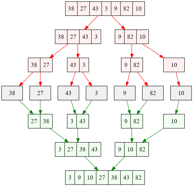


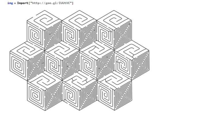
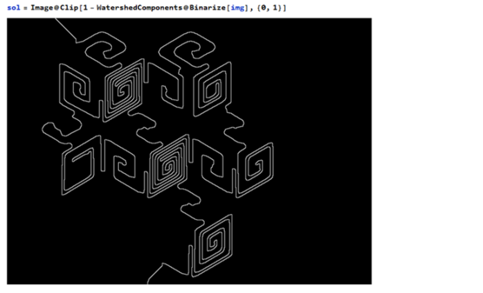
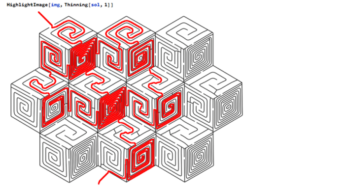
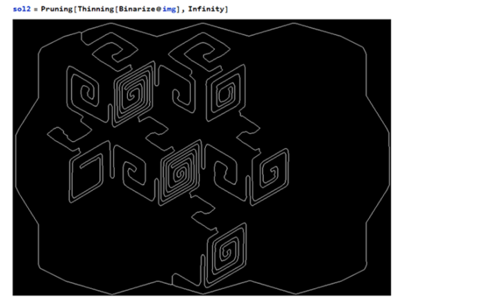
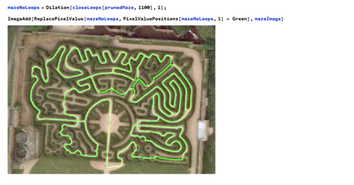
 The maze can be navigated by eliminating any loops
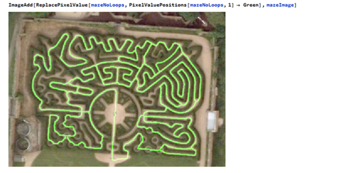
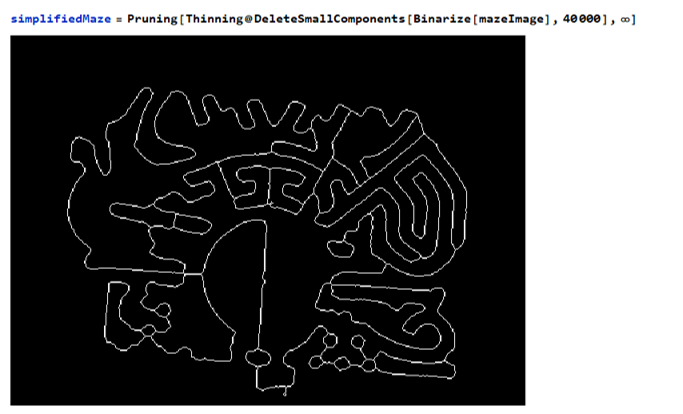
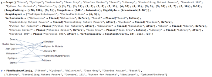
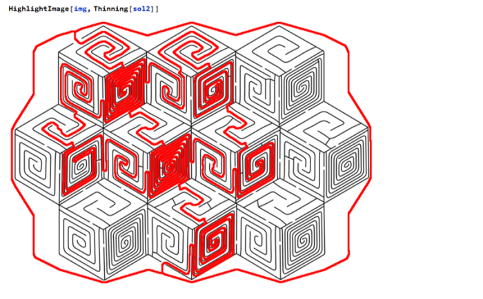
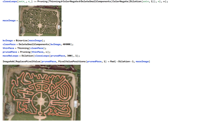
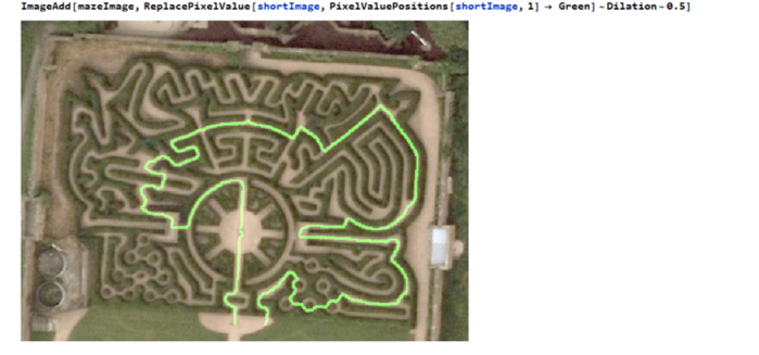
 Now we have a graph to navigate through the maze. Finding the shortest path through the maze is now possible !
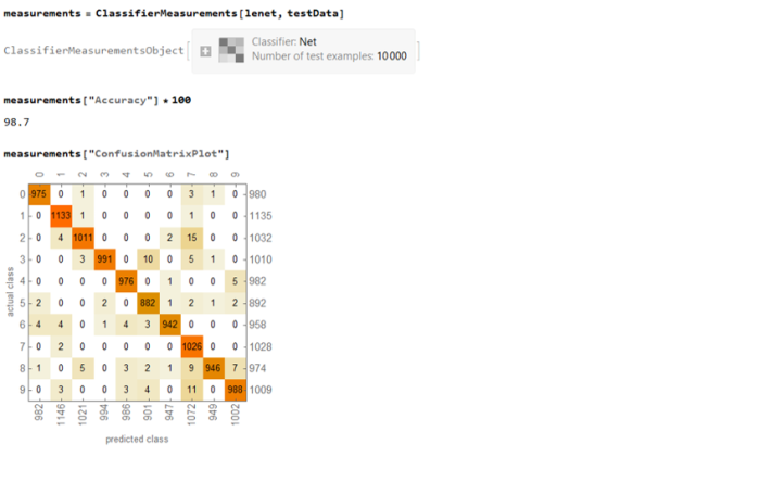
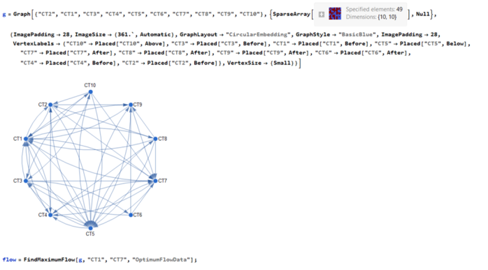
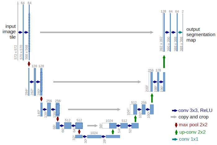
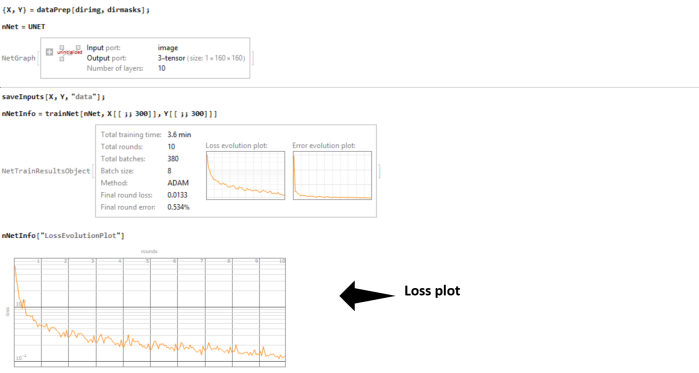
 The network and its structure is uninitialized in the beginning. The great thing about Wolfram Language is that like other expressions, the network itself is a symbolic expression and hence lends itself to symbolic manipulations !!
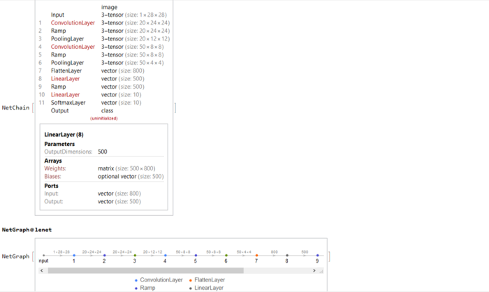
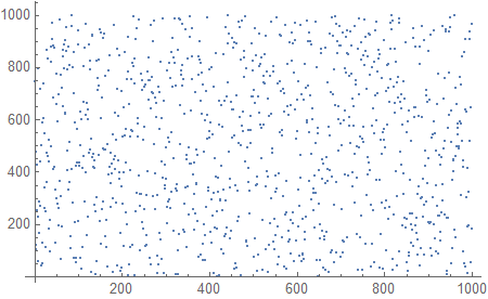
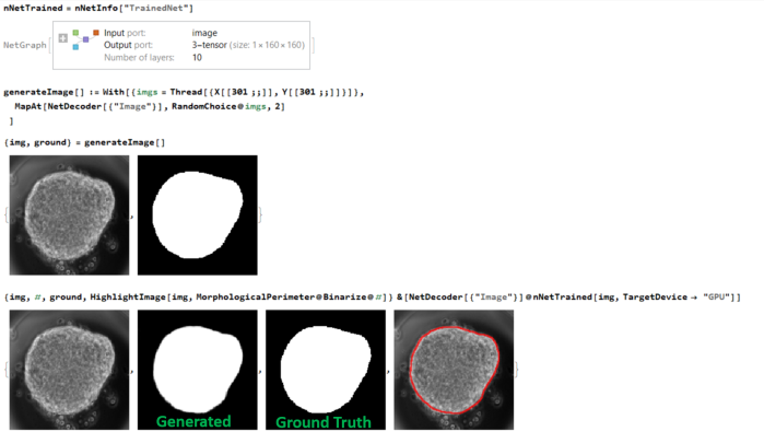
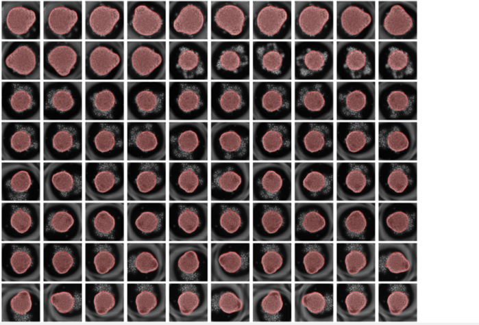
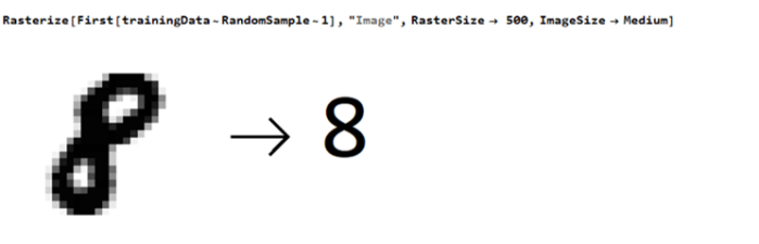
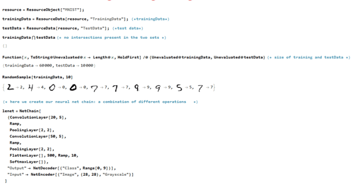
 random images from the
 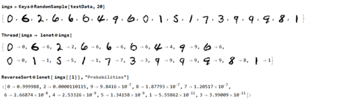 The neural net
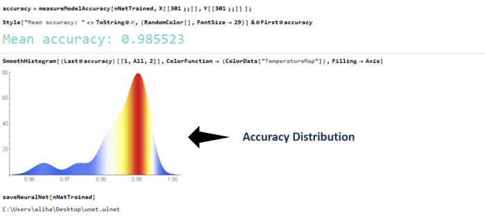